Full Disclosure

OK, before we go on I'm warning you: we're going to talk about Big-O notation. I know, I know, you hated it when you were in school, or, you've never heard of it. Bear with me. We're going to talk about it because it matters. In fact, selecting an algorithm with improved the Big-O performance is often the most effective optimization available, far more than picking a better implementation of a library or moving to faster hardware.

Motivation

Once, a client called me to consult on purchasing a larger server to improve database performance. The client had a substantial existing database with tens of thousands of records summarized in a daily report. The reports had grown until they took more than 16 hours to run, meaning that the client couldn't run them overnight anymore. (This was back in the early 90s.) The reports were essential to their business, driving decisions made each day. Not having the report meant they lacked information they used to guide business decisions, so I was called in to spec fast enough hardware to run the report overnight. The sysadmin walked me through the custom software and how it was used. I asked if I could login to the system. Not a problem. I entered a command and suggested we go to lunch. When I got back from lunch I asked the operator to run the report. Within 5minutes the report was on the screen. "Oh, no, we cannot have canned reports. We need dynamic information based on what happened yesterday." "Look at the report more carefully," I replied. It was a dynamic report.

Big-O Analysis

How did I do it? The report generation performed an outer join on a tables without an indexes. The command I entered over lunch created indexed those tables and changed the Big-O performance from $latex O(N^{2})$ to $latex O(N\log_{2}(N)$.

To scan all the records until a match was found, on average you read half the records which takes time proportional to $latex N$. Let's take a moment and think about this. Assume the operation took some constant number of milliseconds for initialization, e.g. to connect to the database. Call that constant amount of time $latex b$. For every record we read, it takes an average of some other number of milliseconds, call it $latex a$.

To summarize what we've stated so far about the time to read records:

1. To read one record takes the required constant setup time plus the time to read one record, which is $latex t(1)=a+b$.
2. Reading two records requires the constant setup time plus the time to read two records, $latex t(2)=2a+b$.
3. Reading an arbitrary number of records, say $latex N$, takes $latex t(N)=a N+b$.

Big-O notation disregards constant offsets and constant coefficients, because the purpose of Big-O notation is to discuss what happens to a function with a really large number of data elements. And for large enough $latex N$, the type of function, e.g. constant, logarithmic, linear, log-linear, etc., always swamps the additive and multiplicative constants.

Big-O Concept

The idea of Big-O notation is that how an algorithm performs with a large number of elements matters; if you have 2 elements, pretty much any algorithm is going to be OK. (It turns out that there are algorithms that perform poorly for a large number of elements but perform significantly better for a small number of elements, say $latex N\le 100$.)

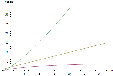
The ranking of Big-O notation, from best to worst is:

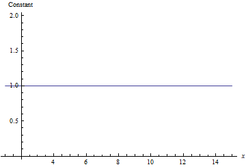
1. $latex O(1)$
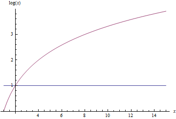
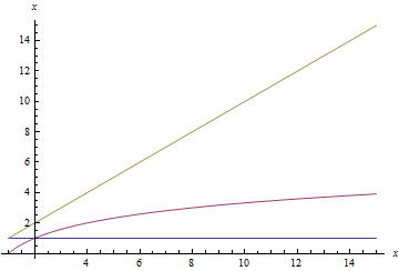
2. $latex O(\log_{2}(x))$
3. $latex O(x log_{2}(x))$
4. Polynomial
   1. $latex O(x^{2})$
   2. $latex O(x^{3})$
   3. $latex O(x^{m})$
5. $latex O(\exp(x))$
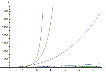
6. $latex O(x!)$

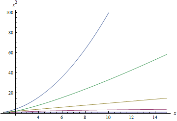
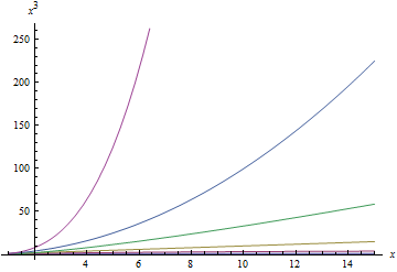
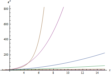
Below is a sequence of plots that plot each of the above functions. When a function is plotted, all better functions are also plotted for comparison. Note that the scale on the $latex y$-axis changes with each plot.

Putting it together

Recapping, we know:

• The time to read $latex N$ records is $latex t(N)=a N +b$.
• Big-O notation disregards additive constants and constant coefficients.

Putting these together tells us that, in Big-O notation, it takes $latex O(N)$ to read $latex N$ records. For each record read, we must compare that one records against all the other records, which means reading them again, so we need $latex O(N)$ to read all the records times $latex O(N)$ to read all the records for comparison, which gives us $latex O(N) * O(N) \Rightarrow O(N^{2})$.

How Bad is $latex O(N^{2})&s=1$?

All right, what they were doing was $latex O(N^{2})$, how bad can that be? For the sake of argument, say the client's database had 10,000 records, that is $latex N=10^{4}$. Because the process was $latex O(N^{2})$ that means the processing time was proportional to $latex 10^{4}*10^{4}=10^{8}$. We know that the total processing time was 16hr. That gives:

$latex \frac{16hr}{10^{8}record}\approx\frac{0.5ms}{record}&s=2$.

The Fix

By indexing the data, a binary search, $latex O(\log_{2}(N))$, can be used instead of the linear search, $latex O(N)$ on each record, giving use $latex $latex O(N) * O(\log_{2}(N)\Rightarrow O(N\log_{2}(N)$. Using $latex N=10^{4}$ with the time for each record as 0.5ms, this gives

$latex 10^{4}\log_{2}(10^{4})*0.5ms\approx 66s&s=1$

From 16hr to 66seconds! Since the actual report took about 5min, we know there was a constant offset and constant coefficient not accounted for in Big-O notation. But WOW!

What does maintaining the indexes cost? In general, insertion into an unsorted list is $latex O(1)\approx 0.5ms$, whereas insertion into a sorted list is $latex O(\log(N))\approx 7ms$ for each inserted record. Not too bad.

Recommended Reading

[amazon_link id="0262033844" target="_blank" ]Introduction to Algorithms[/amazon_link]

[amazon_image id="0262033844" link="true" target="_blank" size="medium" ]Introduction to Algorithms[/amazon_image]